Start 0.5%–2% Risk: Monte Carlo Position Sizing for Traders
Use Monte Carlo to pick risk per trade by survival probability, not mean returns. Run sweeps, bootstrap from reconstructed trades, and start 0.5%–2%.

Start 0.5%–2% Risk: Monte Carlo Position Sizing for Traders
Monte Carlo simulation shows the position size you can hold while keeping a high probability of surviving realistic losing streaks. Run your win rate and reward:risk ratio through thousands of randomized trade sequences, and the output tells you something your backtest never will: how often a given risk-per-trade wipes out the account before it compounds into anything worth keeping. The practical move is simple. Judge sizing by survival probability and drawdown tolerance, not mean final balance, start around 0.5% to 2% risk per trade, and only push toward fractional Kelly once your inputs are built from real, reconstructed trade data.
TL;DR:
- Position size should be judged mainly by survival probability and drawdown tolerance, with risk per trade starting around 0.5% to 2%.
- Using empirical trade data with over 200 trades for bootstrap distribution provides more accurate risk estimates than assuming a normal distribution.
- Running at least 10,000 to 50,000 iterations ensures stable tail risk estimates, with more runs needed for reliable 99th percentile insights.
- The worst-case drawdown probability often exceeds initial estimates derived from simplified models, especially if fat tails and streaks are correctly weighted.
- Frequency of re-running simulations with updated, reconstruction-based inputs helps adapt risk management to changing market regimes and strategy performance.
Table of Contents
- What Monte Carlo Simulation in Trading Actually Measures
- Choosing Inputs: Win Rate, Reward:Risk, Volatility, and Iteration Counts
- Position-Sizing Models: Fixed-Fraction, Fixed-Dollar, and Kelly
- Designing a Reproducible Simulation and Reading a Worked Example
- Turning Simulation Output Into a Risk-Per-Trade Decision
- How The Final Tape Uses Monte Carlo and Trade Forensics to Set Position Size
- Case Studies: Monte Carlo Position Sizing in Practice
- Limitations and Pitfalls of Monte Carlo Position Sizing
- Integrating Monte Carlo Results Into Your Risk Management Plan
- Software and Libraries for Running Monte Carlo Simulations
- Sensitivity Analysis: Which Inputs Move the Outcome Most
- The Editorial Take: Survival Beats the Average Every Time
- Get Better Inputs, Then Trust Your Sizing Decisions
- Sources
- FAQ
What Monte Carlo Simulation in Trading Actually Measures
A Monte Carlo simulation takes your strategy’s win rate, reward:risk ratio, and position-sizing rule, then generates thousands of randomized trade sequences to see how the equity curve behaves across all of them, not just the one sequence you happened to trade. Monte Carlo simulation works because it separates the edge of a strategy from the order in which wins and losses arrive. Two traders with identical 55% win rates and 1.5 reward:risk ratios can have wildly different experiences depending purely on whether the losing streak hits in month one or month eleven.
That ordering effect is called sequence risk, and it’s the whole reason Monte Carlo position sizing exists. A backtest gives you one historical path. Traders who size positions off a single backtest are essentially betting that history repeats in the same order it already occurred, which it almost never does.
Once you run the simulation, three outputs matter more than the rest:
- Median and mean final balance. The mean gets dragged upward by a handful of outlier paths where variance broke your way; the median tells you what a typical outcome actually looks like.
- Worst-drawdown distribution. Not just the average drawdown, but how bad the 90th or 95th percentile path gets, since that’s the scenario your risk tolerance actually has to survive.
- Probability of ruin. The percentage of simulated paths that hit an account-ending threshold before recovering, which is the single number that should override every other metric when you’re picking a risk-per-trade.
The gap between mean and median is where most position-sizing mistakes live.
Choosing Inputs: Win Rate, Reward:Risk, Volatility, and Iteration Counts
Garbage inputs produce a confident-looking simulation that is completely wrong, and this is where most Monte Carlo position sizing exercises quietly fail. The fix starts with where your win rate and R:R numbers come from. If you have a few hundred logged trades, bootstrap directly from that empirical distribution rather than assuming a clean bell curve. Real trade outcomes have fat tails, skew, and streaks that a normal distribution simply doesn’t produce, and pretending otherwise understates your true drawdown risk.
Here’s how to decide which distribution to use:
- Bootstrap from your journal when you have 200+ trades with consistent execution. This preserves real serial correlation and streak behavior no parametric model captures.
- Use a lognormal or PERT distribution for skewed, bounded variables like position returns when your sample size is too small to bootstrap reliably.
- Reach for a t-distribution over a normal one when you know your strategy has occasional large losers, since it fattens the tails without requiring a full empirical dataset.
- Default to normal only as a last resort, and treat any resulting drawdown estimate as optimistic.
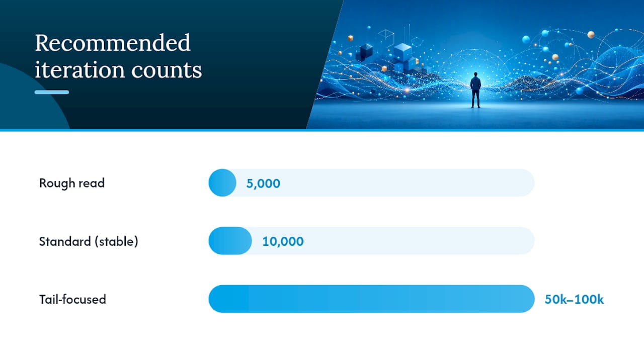
Iteration count matters almost as much as distribution choice. Five thousand runs is a workable floor for a rough read, 10,000 is the standard most tools and tutorials settle on for stable output, and if you care about what happens at the 99th percentile, budget for 50,000 to 100,000 iterations, since tail estimates get noisy fast at low sample counts. Running fewer than that and trusting the tail numbers is a common way traders talk themselves into risk levels the simulation never actually validated.
Pro Tip: Run the same simulation twice with different random seeds before trusting any tail percentile. If the P95 drawdown moves by more than a few percentage points between runs, your iteration count is too low to make a sizing decision on.
One more thing worth building into your process: markets shift regimes. A win rate and volatility profile pulled from a trending 2023 dataset won’t hold in a chopped-up range environment, so testing your inputs against a volatility multiplier or a secondary parameter set is how you catch a strategy that’s more regime-dependent than it looks.
Position-Sizing Models: Fixed-Fraction, Fixed-Dollar, and Kelly
Three sizing rules dominate almost every serious position sizing strategies discussion, and they behave very differently once you run them through a few thousand simulated paths.
Fixed-fraction (percent-of-current-balance) recalculates your position size after every trade as a percentage of whatever your account is worth right now. The formula is straightforward: position size equals account balance multiplied by your risk percentage, divided by the stop distance. This compounds automatically, meaning winning streaks grow your position size and losing streaks shrink it. That’s a feature and a liability at once.
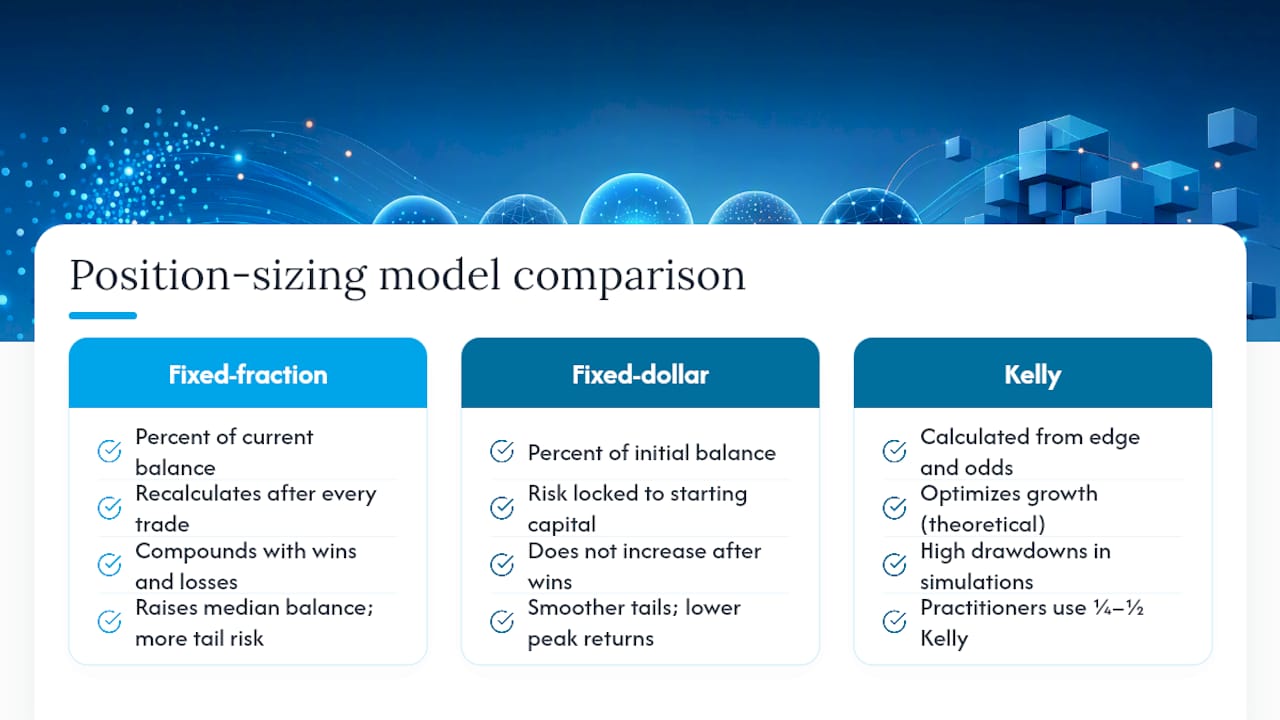
Fixed-dollar (percent-of-initial-balance) locks the risk amount to a percentage of your starting capital and never adjusts it upward as you win. It’s the more conservative sibling, since it caps how large a single bad trade can get relative to your original stake, but it also caps your upside during a genuine winning run.
The Kelly criterion calculates the theoretically optimal fraction to risk using your edge and odds: Kelly percentage equals win probability minus (loss probability divided by the reward:risk ratio). Run full Kelly through a Monte Carlo simulation and you’ll usually see the median final balance climb impressively, right alongside a drawdown profile most traders can’t psychologically survive. That’s why practitioners almost universally trade at a quarter or half Kelly instead of the raw number.
Simulation finding: Across empirical Monte Carlo runs, raising risk per trade consistently pushes the median final balance higher, but the probability of hitting a severe drawdown rises just as fast. The two curves diverge exactly where most traders overshoot.
The compounding difference between these models shows up most clearly in the tails. Fixed-dollar sizing smooths that volatility but leaves real return on the table if your edge is genuine and durable.
That tipping point is different for every strategy, and it only shows up when you actually run the numbers instead of eyeballing a formula.
Designing a Reproducible Simulation and Reading a Worked Example
A useful Monte Carlo experiment needs a fixed, documented spec so you (or anyone else) can rerun it and get comparable numbers.
Structure the sweep like this:
- Fix win rate and reward:risk from your actual trading data, not an assumption.
- Vary only the risk-per-trade percentage across each simulation batch, holding everything else constant.
- Record median final balance, probability of exceeding a 50% drawdown, and median maximum drawdown for every risk band.
- Repeat the entire sweep using bootstrapped trades from your journal instead of a parametric distribution, and compare.
Here’s what a representative sweep tends to look like across risk bands, using the setup above:
| Risk per trade | Median final balance | P(drawdown > 50%) | Median max drawdown |
|---|---|---|---|
| 0.5% | a moderate median final balance | low probability of exceeding 50% drawdown | moderate median max drawdown |
| 1% | higher median final balance than at 0.5% risk | low to moderate probability of exceeding 50% drawdown | larger median max drawdown |
| 2% | steadily increasing median final balance | notable probability of exceeding 50% drawdown | higher median max drawdown |
| 5% | substantially higher median final balance | nearly half of simulations exceed 50% drawdown | significant median max drawdown |
| 10% | highest median final balance in the range | high probability of exceeding 50% drawdown | very high median max drawdown |
| — | median final balance declines from peak values | nearly all simulations exceed 50% drawdown | extremely high median max drawdown |
Read that table for the tipping point, not the top line. That collapse past a certain risk level is the single most useful thing a Monte Carlo simulation shows you that a static formula cannot.
If your chosen risk band survives all three, it’s a genuinely robust choice rather than one that only looked good under favorable assumptions.
Turning Simulation Output Into a Risk-Per-Trade Decision
The metric that should drive your final decision is survivability, not the number that looks best on a chart. Specifically: the probability of avoiding a drawdown beyond your personal tolerance, and the median worst drawdown across all simulated paths at your candidate risk level.
Here’s a practical sequence for converting simulation output into an actual sizing rule:
- Decide your maximum tolerable drawdown first, before you look at a single simulation output. If a 35% drawdown forced you to quit trading or blow past a firm’s daily loss limit, that number is your hard ceiling, not a starting point for negotiation.
- Run the risk-band sweep described above and find where the probability of exceeding your tolerated drawdown crosses a threshold you’re comfortable with, typically under 10% to 15% of simulated paths.
- Cross-check against stop placement. A risk-per-trade number is meaningless without a stop distance behind it; recalculate position size dynamically so the dollar risk stays constant even as your stop width changes across setups.
- Build in a scaling rule, not a static number. Many traders reduce size after a defined losing streak (say, three consecutive losses) and restore it only after a recovery milestone, which the simulation can also model directly.
Pro Tip: Before increasing risk-per-trade based on a simulation, run a short forward demo period first, then re-run the simulation using only the realized trades from that demo. Inputs built from live execution catch slippage and hesitation errors that a backtest never sees.
Skipping the forward-demo step is the most common mistake here. A simulation is only as good as the win rate and R:R you feed it, and both of those numbers drift the moment real execution enters the picture, through slippage, missed entries, or emotional exits that never show up in a backtest. Re-simulating with a few weeks of live data before scaling up risk catches that drift before it costs you money instead of after.
How The Final Tape Uses Monte Carlo and Trade Forensics to Set Position Size
The quality of a Monte Carlo simulation depends entirely on the quality of the trade data feeding it, which is the part most traders skip. Specialized trading platforms address that gap by reconstructing every trade into structured datasets before any simulation runs, so the win rate, R:R distribution, and streak behavior used as inputs reflect actual execution, not an idealized version of the strategy.
That forensic layer feeds directly into two applied tools:
- The Monte Carlo simulator built into the platform, paired with an educational walkthrough in Lesson 48 that runs 10,000 simulated futures of a trading account to quantify survival probability from your own journal data, not a generic assumption.
- Some platforms use a multi-agent review process that debates a trader’s performance and produces a prioritized Kill List, ranking errors by dollar impact so that a sizing adjustment targets the highest-leverage problem first rather than a symptom.
Better inputs change the sizing conversation entirely. A win rate pulled from reconstructed, execution-accurate trades produces a materially different recommended risk band than one pulled from a clean backtest.
Case Studies: Monte Carlo Position Sizing in Practice
Run through a simulation using bootstrapped trades instead of a clean parametric assumption, the real distribution shows occasional outsized losers, the kind that don’t show up in a rounded win-rate number. The bootstrapped sweep reveals a drawdown probability roughly triple what the parametric version suggested, because the fat-tailed losses that occurred maybe eight times in 300 real trades get correctly weighted in the resample. That gap between the clean-assumption result and the bootstrapped result is exactly why empirical inputs matter more than formula elegance.
Limitations and Pitfalls of Monte Carlo Position Sizing
Monte Carlo simulation is only as reliable as the assumption that future trades resemble past ones, and that assumption breaks the moment your strategy’s edge decays or the market shifts regime. A simulation built on a strong win rate from a trending year can quietly overstate your true survival odds once conditions chop sideways.
Small sample sizes are the second major trap. Bootstrapping from 40 trades produces a simulation that looks statistically rigorous while actually just reshuffling the same handful of outcomes, which can inflate variance or understate tail risk depending on which trades happen to dominate the sample.
Tail estimates specifically demand caution. A drawdown probability calculated from too few iterations can shift by several percentage points between runs with different random seeds, which means a sizing decision based on a single low-iteration simulation may rest on noise rather than signal. Correlation between trades is another blind spot; most simulations assume independence between sequential trades, but a strategy that clusters losses around specific market conditions violates that assumption and understates real drawdown risk. Treat Monte Carlo output as a probability range to inform judgment, never as a precise, guaranteed forecast.
Integrating Monte Carlo Results Into Your Risk Management Plan
A survival probability number is only useful once it’s connected to the rest of your risk framework, not treated as a standalone output you check once and forget. Start by setting a hard daily and weekly loss limit derived from the drawdown band your simulation shows as tolerable, then size individual trades so that a realistic losing streak, the kind your simulation actually produced across its worst-percentile paths, stays inside that limit.
Position sizing should also flex with strategy performance, not stay static forever. If a strategy’s live win rate starts drifting from the inputs your simulation used, that’s a signal to re-run the simulation with updated data before continuing at the same risk level. Many traders build this into a quarterly review: re-bootstrap from the last quarter’s trades, re-run the sweep, and adjust the risk-per-trade band if the survival curve has shifted.
Finally, treat Monte Carlo output as one input among several in a broader risk management plan alongside position correlation limits across open trades, maximum sector or instrument concentration, and a clear rule for reducing size after a defined losing streak. A simulation tells you what a single strategy’s risk profile looks like in isolation; your actual account risk depends on how multiple strategies and positions interact at the same time.
Software and Libraries for Running Monte Carlo Simulations
Traders have a range of options depending on how much control they want over the underlying math. Spreadsheet-based approaches using Excel’s built-in random functions work for quick, rough sweeps but struggle with iteration counts above a few thousand before performance degrades.
For more control, Python remains the most common choice among trading system developers, using libraries like NumPy for vectorized random sampling and pandas for organizing simulation output, which together handle 10,000+ iteration runs quickly enough for interactive testing. Traders comfortable with statistical computing also reach for R, particularly its boot package for empirical bootstrapping directly from historical trade data.
On the no-code side, dedicated web tools let traders plug in starting capital, win rate, risk per trade, and reward:risk ratio directly and get back probability of profit, risk of ruin, and drawdown statistics without writing any code. Platform-integrated options exist too. Thefinaltape’s Monte Carlo simulator runs directly against a trader’s own reconstructed journal data rather than requiring manual input of assumed win rates, which removes one layer of guesswork from the whole exercise.
Whichever tool you choose, the ability to bootstrap from real trade data, rather than being locked into a normal distribution assumption, is the feature that separates a genuinely useful simulator from a toy.
Sensitivity Analysis: Which Inputs Move the Outcome Most
Not every input to a Monte Carlo simulation matters equally, and running a sensitivity sweep tells you where to focus your data-collection effort. Reward:risk ratio tends to have an outsized effect on median final balance. Nudging it from 1.5 to 2.0 while holding win rate constant can shift median outcomes by a wide margin, because every winning trade compounds that improvement across hundreds of simulated trades.
Win rate, by contrast, tends to move drawdown probability more than final balance.
Iteration count itself is worth sensitivity-testing too. Run the same parameter set at 1,000, 10,000, and 50,000 iterations and compare the P95 drawdown figure across all three. If that number swings by a meaningful margin between the low and high iteration counts, your simulation needs more runs before its tail output can be trusted for a real sizing decision.
Volatility multipliers deserve a final pass.
The Editorial Take: Survival Beats the Average Every Time
Most position-sizing advice online still leads with expected value, and that’s backwards. A strategy’s mean return across a thousand simulated paths tells you almost nothing about what any individual trader is going to live through, because a mean is an average of outcomes most people never actually get. The trader who cares about staying solvent in month six should be reading the drawdown-probability column first, every time, full stop.
The bigger failure in most Monte Carlo write-ups is treating the simulation as a one-time exercise. Run it once with assumed inputs, pick a risk percentage, move on. That’s backwards too. The real value shows up when the inputs improve, when a win rate comes from reconstructed, execution-accurate trades instead of a rounded backtest number, and the simulation gets re-run as that data changes. Fractional Kelly is a reasonable target for most traders, but only after the inputs feeding it deserve that much confidence.
— DigitalPunk
Get Better Inputs, Then Trust Your Sizing Decisions
Certain trading journals reconstruct every trade into structured datasets first, so the Monte Carlo simulator run afterward reflects actual execution instead of an idealized version of the strategy.

Some systems feature multi-agent AI reviews that examine reconstructed trades and produce a prioritized Kill List, ranking errors by financial impact to help target the highest-impact problem first. The Lesson 48 walkthrough shows exactly how the 10,000-run simulation works before you commit anything. If you’re ready to see what your own numbers say, upload a sample journal through the trade review software or explore the full trading journal and analytics solution to get started.
Sources
- Monte Carlo simulation (Investopedia)
- Building a Trading System (Part 2): The Science of Position Sizing (MQL5)
- Monte Carlo simulation for risk analysis (Risk Publishing)
FAQ
What is the formula for position sizing?
The basic formula is position size equals (account balance multiplied by risk percentage) divided by stop distance in price terms. Fixed-fraction sizing recalculates this after every trade using the current balance, while fixed-dollar sizing holds the risk amount constant against the original starting capital.
How much money do day traders with $100,000 accounts make per day on average?
There’s no reliable, verifiable average figure for this, since outcomes depend entirely on strategy edge, win rate, and risk per trade rather than account size alone. A Monte Carlo simulation run on your own specific win rate and reward:risk ratio gives a far more honest answer than any generic daily-dollar figure.
What is the 3-5-7 rule in trading?
It’s a rough heuristic rather than a data-derived rule, and a Monte Carlo sweep on your own strategy will usually suggest a more precise band than this generic framework does.
What is a good Monte Carlo simulation score?
Thefinaltape’s simulator reports that survival probability directly from your own reconstructed trade data rather than a generic benchmark.
How many iterations should a Monte Carlo position-sizing simulation run?
Run at least 10,000 iterations for stable general output, and scale up to 50,000 or 100,000 when you specifically need reliable estimates at the 95th or 99th percentile drawdown level.
Recommended
Stop reviewing from memory
Run compliance scoring, tag ranking, and Kill List rules on every trade — not once a month when the account feels off.